User Manual

Home News Downloads Tutorials User Manual Reference Manual Developer Manual Forums Team Members Future Work FAQ Links

Topographica spatial coordinate systems Topographica allows simulation parameters to be specified in units that are independent of the level of detail used in any particular run of the simulation. To achieve this, Topographica provides multiple spatial coordinate systems, called Sheet and matrix coordinates. Sheet coordinates Quantities in the user interface are expressed in Sheet coordinates. A Topographica Sheet is a continuous abstraction of a finite, two-dimensional array of neural units. A Sheet corresponds to a rectangular portion of a continuous two-dimensional plane. The default Sheet has a square area of 1.0 centered at (0.0,0.0): Locations in a Sheet are specified using floating-point Sheet coordinates (x,y) contained within the Sheet's BoundingBox. The thick black line in the figure above shows the BoundingBox of the default Sheet, which extends from (-0.5,-0.5) to (0.5,0.5) in Sheet coordinates. Any coordinate within the BoundingBox is a valid Sheet coordinate. Matrix coordinates Although it is possible to do some computations using analytic representations of the continuous Sheet, in practice, Sheets are typically implemented using some finite matrix of units. Each Sheet has a parameter called its density, which specifies how many units (matrix elements) in the matrix correspond to a unit length in Sheet coordinates. For instance, the default Sheet above with a density of 5 corresponds to the matrix on the left below: Here, the 1.0x1.0 area of Sheet coordinates is represented by a 5x5 matrix, whose BoundingBox (represented by a thick black outline) corresponds exactly to the BoundingBox of the Sheet to which it belongs. Each floating-point location (x,y) in Sheet coordinates corresponds uniquely to a floating-point location (r,c) in floating-point matrix coordinates, and vice versa. Individual units or elements in this array are accessed using integer matrix index coordinates, which can be calculated from the matrix coordinate (r,c) as (floor(int(r)),floor(int(c))). For the example shown, the center of the unit with matrix index (0,1) is at location (0.5,1.5) in matrix coordinates and (-0.2,0.4) in Sheet coordinates. Notice that matrix and matrix index coordinates start at (0.0,0.0) in the upper left and increase down and to the right (as is the accepted convention for matrices), while Sheet coordinates start at the center and increase up and to the right (as is the accepted convention for Cartesian coordinates). The reason for having multiple sets of coordinates is that the same Sheet can at another time be implemented using a different matrix specified by a different density. For instance, if this Sheet had a density of 10 instead, the corresponding matrix would be: Using this higher density, Sheet coordinate (-0.2,0.4) now corresponds to the matrix coordinate (1.0,3.0). As long as the user interface specifies all units in Sheet coordinates and converts these to matrix coordinates appropriately, the user can use different densities at different times without changing any other parameters. Connection fields Units in a Topographica Sheet can receive input from units in other Sheets. Such inputs are generally contained within a ConnectionField, which is a spatially localized region of an input Sheet. A ConnectionField is bounded by a BoundingBox that is a subregion of the Sheet's BoundingBox. The units contained within a ConnectionField are those whose centers lie within that BoundingBox. 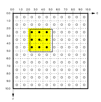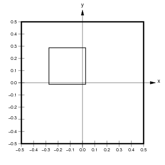For instance, if the user specifies a ConnectionField with Sheet bounds from (-0.275,-0.0125) to (0.025,0.2885) for a sheet with a density of 10, the corresponding matrix coordinate bounds are (5.125,2.250) to (2.125,5.250): Here the medium black outline shows the user-specified ConnectionField BoundingBox in matrix and Sheet coordinates. The units contained in this ConnectionField are (4,2) to (2,4) (inclusive; shown by black dots with a yellow background). Notice that the Sheet area of the ConnectionField will not necessarily correspond exactly to the user-specified BoundingBox, because the matrix is discrete. Note that a ConnectionField is similar to the biological concept of a receptive field (RF), but the two concepts are the same only for models with one input sheet and one cortical sheet. When there is more than one hierarchical level, the ConnectionField of a top-level unit is a set of weights on the previous Sheet, while the receptive field is an area of the input sheet to which the unit responds. Thus a ConnectionField is a lower-level concept than a receptive field, and RFs can be thought of as constructed from CFs. Edge buffering If every Sheet has the default 1.0x1.0 area, units near the border of higher-level Sheets will have ConnectionFields that extend past the border of lower-level Sheets. This ConnectionField cropping will often result in artifacts in the behavior of units near the border. To avoid such artifacts, lower-level Sheets should usually have areas larger than 1.0x1.0. For instance, assume that Sheets have a 1.0x1.0 area. If a higher level sheet U has a ConnectionField BoundingBox of size 0.4x0.4 on lower-level Sheet L, neurons near the border of U will have up to 0.2 in Sheet coordinates cut off of their ConnectionFields. 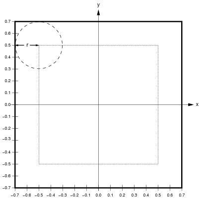To prevent this, the BoundingBox of L can be extended by 0.2 in Sheet coordinates in each direction: Here, the thick black line shows the calculated size of L to avoid edge cropping, and the dotted line shows the size of U for reference. If L were the size of U, up to three quarters of the ConnectionField of units in U near the border would be cut off. With the size of L extended as shown, all units in U will have full ConnectionFields. Thus when calculating the behavior of U, the extended L will work as if L were infinitely large in all directions. This approach is appropriate for avoiding edge effects when modeling a small patch of a larger system. Of course, this technique cannot help you avoid such cropping for lateral connections within U or feedback connections from areas above U. In some simulators, periodic boundary conditions can be enforced such that such connections wrap around like a torus, avoiding these issues. However, such wrapping is not practical in Topographica, which focuses on drawing realistic input patterns like photographs, which cannot be rendered properly on a torus. Technical details In some cases, the details of representing a Sheet with a matrix of a certain density can be more complex than described above, because it is possible to specify a bounds and density combination that cannot be realized exactly. For this reason, the quantities set by the user are called nominal_density and nominal_bounds, and the true bounds and density are calculated from these. For instance, consider requesting that a Sheet have bounds of BoundingBox(radius=0.3), and density of 7. Such an area (a 0.6 x 0.6 square) cannot be tiled exactly by 7 units per 1.0 length. When a sheet is created, the density will be adjusted so that the requested sheet bounds (and thus the overall area) is respected. In this example, the Sheet would have an actual density of 6.67 (the closest value to tile the plane exactly; see SheetCoordinateSystem). This approach was chosen so that whenever the density is changed, the simulation remains the best possible approximation of the requested area. However, because the bounds do not have to be square, there can be an additional complication for certain bounds and densities. Consider the example above, but instead with rectangular bounds given by BoundingBox(points=((-0.3,-0.5),(0.3,0.5))). This time, the y dimension would be tiled exactly by a density of 7, but the x dimension would not. This problem could be solved by allowing a Sheet to have different densities in each dimension (i.e. an xdensity and a ydensity); indeed, the SheetCoordinateSystem underlying a Sheet does not require that the xdensity and ydensity are equal. However, for a Sheet itself, it is simpler for the density to be equal in both dimensions. To solve the problem above, then, we take the bounds's x-width and calculate an xdensity from this (as described for the previous example), and make the ydensity exactly equal to this by adjusting the top and bottom bounds. In our example, the top bound would be adjusted to 0.525, and the bottom to -0.525---the closest bounds allowing a density of 6.67 to tile the dimension exactly. In summary, the bounds specified for a Sheet are respected, but the density may be adjusted so that the plane is tiled exactly. In certain cases where it is not possible to have the same density in the y direction as in the x direction with the specified bounds, the top and bottom bounds are adjusted so that the densities can remain equal. This is an "x-bounds-master" approach; futher discussion of this and alternatives is available in SheetCoordinateSystem.

Hosted by: James A. Bednar (jbednar@inf.ed.ac.uk) Last update: Thu Sep 4 0:54:24 BST 2008.