Topographica Command Line
The GUI interface of Topographica provides the most commonly used plots and displays, but it is often useful to be able to manipulate the underlying program objects interactively. The Topographica command prompt allows you to do this easily, using the same syntax as in Topographica scripts. This section describes the basic IPython-based interactive prompt that is available whenever Topographica starts. Topographica also supports the more full-featured IPython Notebook interface using a web browser, which supports all of the same commands and also provides interactive visualization facilities similar to those in the GUI (but more flexible). See the Tutorials for examples of using the notebook interface.
The command prompt gives you direct access to Python, and so any expression valid for Python can be entered. For instance, if your script defines a Sheet named V1, you can display and change V1’s parameters using Python commands:
[cloud]v1cball: topographica -i ~/Documents/Topographica/examples/tiny.ty

Welcome to Topographica!

Type help() for interactive help with python, help(topo) for general
information about Topographica, help(commandname) for info on a
specific command, or topo.about() for info on this release, including
licensing information.


topo_t000000.00_c1>>> topo.sim['V1'].density
               Out[1]:5.0

topo_t000000.00_c2>>> topo.sim['V1'].output_fns[0]
               Out[2]:PiecewiseLinear(lower_bound=...)

topo_t000000.00_c3>>> from topo.transferfn import *

topo_t000000.00_c4>>> topo.sim['V1'].output_fns=[IdentityTF()]

topo_t000000.00_c5>>> topo.sim['V1'].output_fns[0]
               Out[5]:IdentityTF(name=...)

topo_t000000.00_c6>>> topo.sim['V1'].activity
               Out[6]:
array([[ 0.,  0.,  0.,  0.,  0.],
       [ 0.,  0.,  0.,  0.,  0.],
       [ 0.,  0.,  0.,  0.,  0.],
       [ 0.,  0.,  0.,  0.,  0.],
       [ 0.,  0.,  0.,  0.,  0.]])
...
For very large arrays, numpy will suppress printing the array data to avoid filling your terminal with numbers. If you do want to see the data, you can tell numpy to print even the largest arrays:
topo_t000000.00_c7>>> numpy.set_printoptions(threshold=2**30)
To see what is available for inspection or manipulation for any object, you can use dir():
topo_t000000.00_c10>>> dir(topo.sim['V1'])
               Out[10]:
['_EventProcessor__abstract',
...
 'activity',
 'activity_len',
 'apply_output_fns',
 'bounds',
...]
Note the directory will typically include many items that are not useful to inspect, including those starting with an underscore (_), but it gives a good idea what an object contains. You can also get information about most objects by typing ? after the name, or by using the help() function for more detailed information:
topo_t000000.00_c11>>> PiecewiseLinear?
...
Docstring:
    Piecewise-linear TransferFn with lower and upper thresholds.

    Values below the lower_threshold are set to zero, those above
    the upper threshold are set to 1.0, and those in between are
    scaled linearly.

Constructor information:
Definition: PiecewiseLinear(self, **params)
Docstring:
    Initialize this Parameterized instance.

    The values of parameters can be supplied as keyword arguments
    to the constructor (using parametername=parametervalue); these
    values will override the class default values for this one
    instance.

    If no 'name' parameter is supplied, self.name defaults to the
    object's class name with a unique number appended to it.


topo_t000000.00_c12>>> help(topo.sim['Retina'])

Help on GeneratorSheet in module topo.sheet object:

class GeneratorSheet(topo.base.sheet.Sheet)
 |  Sheet for generating a series of 2D patterns.
 |
 |  Typically generates the patterns by choosing parameters from a
 |  random distribution, but can use any mechanism.
 |
...
 |  Methods defined here:
 |
 |  __init__(self, **params)
 |
 |  generate(self)
 |  Generate the output and send it out the Activity port.
 |
...
 |  ----------------------------------------------------------------------
 |  Data descriptors defined here:
 |
 |  apply_output_fns
 |  Whether to apply the output_fns after computing an Activity matrix.
 |
 |  input_generator
 |  Specifies a particular PatternGenerator type to use when creating patterns.
 |
...
 |  ----------------------------------------------------------------------
 |  Data and other attributes defined here:
 |
 |  src_ports = ['Activity']
 |
...
See the IPython Quick Tutorial for IPython-specific extensions useful from the command prompt.
Recreating results from interactive sessions
While interactive creation and exploration of a simulation can be very helpful, often you will want to create a representation of your simulation that you can use again. One way of doing this is to save an existing simulation that you have already created at the commandline (see save_script_repr for how to save a runnable specification of your simulation (but not its internal state), or save_snapshot for how to save your simulation’s current state). Another way is to create a .ty script file yourself, and then run it with Topographica. As discussed in the Topographica scripts section, exactly the same commands can be entered in a .ty file as at the commandline, and running the .ty file (either by passing it at startup to the topographica program on the commandline, or by passing it as an argument to execfile()) is equivalent to entering its commands manually.
Plotting from the command line
If the GUI is running, you can also plot any vector or matrix in the program:
$ topographica -g ~/Documents/Topographica/examples/tiny.ty
Topographica> topo.sim.run(1)
Topographica> from topo.command.pylabplot import *
Topographica> V1 = topo.sim['V1']
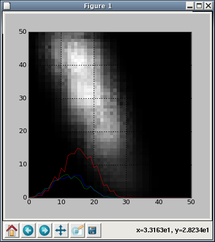
Topographica> matrixplot(V1.activity)
Topographica> vectorplot(V1.activity[0])
Topographica> vectorplot(V1.activity[1])
Topographica> vectorplot(V1.activity[10])
Topographica>
Result:
You can also try replacing matrixplot with matrixplot3d to get a 3D wireframe plot:
Topographica> matrixplot3d(V1.activity)
Result:
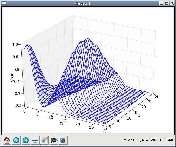
Be sure to try clicking and dragging on the plot, to rotate the viewpoint.
The prompt can also be used for any mathematical calculation or plotting one might wish to do, a la Matlab:
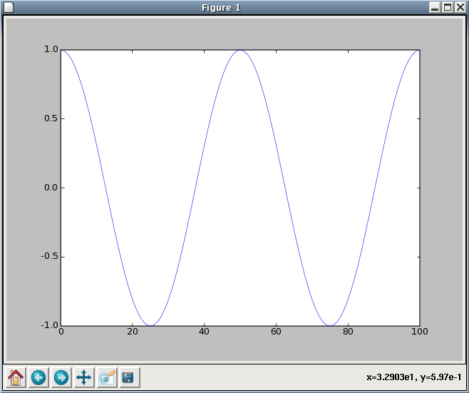
$ topographica -g
Topographica> from numpy import *
Topographica> 2*pi*exp(1.6)
31.120820554943471
Topographica> t = arange(0.0, 1.0+0.01, 0.01)
Topographica> s = cos(2*2*pi*t)
Topographica> from pylab import *
Topographica> plot(s)
[<matplotlib.lines.Line2D instance at 0xb6b1aeac>]
Topographica> show._needmain = False
Topographica> show()
Resulting plot:
See the numpy documentation for more details on the mathematical expressions and functions supported, and the MatPlotLib documentation for how to make new plots and change their axes, labels, titles, line styles, etc.
Saving or accessing Topographica bitmaps
A command save_plotgroup is provided to allow you to automate the process of generating and saving the various bitmap images visible in the Topographica GUI. For instance, to measure an orientation map and save the resulting bitmaps to disk, just do:
Topographica> from topo.command.analysis import measure_or_pref
Topographica> from topo.plotting.plotgroup import save_plotgroup
Topographica> measure_or_pref()
Topographica> save_plotgroup("Orientation Preference")
The name “Orientation Preference” here is just the name used in the Plots menu, and the command “measure_or_pref()” is listed at the bottom of the Orientation Preference window. These names and functions are typically defined in topo/command/analysis.py, and are used to present testing images and store the resulting responses. The command save_plotgroup then uses this data to generate the bitmap images, and saves them to disk.
By default, all output from Topographica goes into Topographica folder in your Documents directory (this can be customized, and is ~/topographica in release 0.9.7 and earlier; see the note about the default output path for more information).
Other examples:
save_plotgroup("Activity")
save_plotgroup("Projection",projection=topo.sim['V1'].projections('Afferent'))
As shown above, some plotgroups (such as Projection) accept optional parameters. Using these commands makes it possible to run simulations without any GUI, for batch or remote processing.
It is also possible to access these bitmaps from the command line, if you want to analyze them rather than save them. For example to see the matrix of values for the OrientationPreference, plus the bounding box in Sheet coordinates, do:
measure_or_pref()
(mat,bbox)=topo.sim['V1'].sheet_views['OrientationPreference'].view()
print mat
print bbox.lbrt()
Imports
In the sample code above, each command is imported (i.e., loaded and declared) from the appropriate file before it is used. Python requires such importing to avoid confusion between similar commands defined in different files; see the Python documentation for more information about imports.
To avoid confusion, we recommend you take advantage of Python’s namespaces (as mentioned earlier in the Imports section of the Topographica Scripts page) when working interactively at the commandline. For instance, pattern.random.UniformRandom is clearly distinct from numbergen.UniformRandom; importing one or the other (or both!) as only UniformRandom (e.g. from numbergen import UniformRandom) could lead to confusion. Of course you might decide that in many cases, using the namespace at the command-line involves too much typing; you are free to use whichever technique you prefer.
Simplifying imports during interactive runs
When working interactively, typing common import lines (such as from topo.command.analysis import measure_or_pref, from the earlier example) can be tedious. Topographica therefore provides the “-a” command-line option, which automatically imports every command in topo/command/*.py. The “-g” option also automatically enables “-a”, so that the commands will be available in the GUI as well. Thus if you start Topographica as “topographica -a” or “topographica -g”, then you can omit the from topo.command... import ... lines above. Still, it is best never to rely on this behavior when writing .ty script files or .py code, because of the great potential for confusion, so please use “-a” only for interactive debugging.
Customizing the command prompt
The contents of the command prompt itself are controlled by the CommandPrompt class, and can be set to any Python code that evaluates to a string. As of 09/2008, the default prompt is topo_t000000.00_c1>>>, where t000000.00 is the current value of topo.sim.time() when the prompt is printed, and the 1 following c is IPython’s record of your command number (IPython caches your input and output in the lists In and Out respectively; the command number allows you to access a specific entry as e.g. In[1]).
You can change the prompt format by doing something like:
from topo.misc.commandline import CommandPrompt
CommandPrompt.set_format('${my_var}>>> ')
where in this case the value of a variable my_var will be checked each time before the prompt is printed. IPython allows the prompt to be configured in many ways; see IPython’s User Manual for full details about what you can pass as an argument to CommandPrompt.set_format in Topographcia.
In addition to the input prompt described above, there is also an output prompt (e.g. Out[3]:) and a continuation prompt (e.g. ....:). You can also customize these in the same way as the input prompt by using the OutputPrompt and CommandPrompt2 classes, respectively, in the same way.
Site-specific customizations
If you have any commands that you want to be executed whenever you start Topographica, you can put them into the user configuration file. For instance, to use the ANSI colors every time, just add these lines to your user configuration file:
from topo.misc.commandline import CommandPrompt
CommandPrompt.format = CommandPrompt.ansi_format
Debugging or verbose messaging
If you want to study exactly how Topographica is operating, e.g. to extend it or control it from the command line, you can consider changing the param.parameterized.min_print_level parameter so that messages will be printed whenever Topographica performs an action. For instance, you can enable verbose messaging by starting Topographica as:
topographica -c "import param" \
-c "param.parameterized.min_print_level=param.parameterized.VERBOSE" ...
Instead of VERBOSE, you can use any of the other message levels defined in parameterized.py, such as DEBUG, which gives even more information (typically much more than is useful).
Controlling the GUI from scripts or the command line
The code for the Topographica GUI is kept strictly separate from the non-GUI code, so that Topographica simulations can be run remotely, automated using scripts, and upgraded to newer graphical interface libraries as they become available. Thus in most cases it is best to ensure that your scripts do not contain any GUI-specific code. Even so, in certain cases it can be very helpful to automate GUI operations using scripts or from the command line, e.g. if you always want to open a standard set of windows for analysis.
For such situations, Topographica provides a simple interface for controlling the GUI from within Python. For instance, to open an Activity window, which is under the Plots menu, type:
import topo
topo.guimain['Plots']['Activity']()
Some menu items accept optional arguments, which can be supplied as follows:
import topo
topo.guimain['Plots']['Connection Fields'](x=0.1,y=0.2,sheet=topo.sim['V1'])
topo.guimain['Plots']['Activity'](normalize=True,auto_refresh=False)
Other examples:
topo.guimain['Plots']['Preference Maps']['Orientation Preference']();

p=topo.guimain['Plots']
p['Activity']();
p['Connection Fields']()
p['Projection']()
p['Projection Activity']()
p['Tuning Curves']['Orientation Tuning']()

topo.guimain['Simulation']['Test Pattern']()
topo.guimain['Simulation']['Model Editor']()
In each case, the syntax for calling the command reflects the position of that command in the menu structure. Thus these examples will no longer work as the menu structure changes; no backwards compatibility will be provided. These commands should be treated only as a shortcut way to invoke GUI menu items, not as an archival specification for how a model works.
Note that if you are doing any of these operations from a Topographica script, it is safest to check first that there is a GUI available, because otherwise the script cannot be executed when Topographica is started without the -g option. Topographica defines the guimain attribute of the topo namespace only when there is a GUI available in this run. Thus if you check to make sure that guimain is defined before running your GUI commands:
if hasattr(topo,'guimain'):
   topo.guimain['Plots']['Activity']()
then your scripts should still work as usual without the GUI (apart from opening GUI-related windows, which would not work anyway).
Additionally, it is possible to script more complex GUI operations. For instance, one can open an Orientation Preference window and request that the map be measured by invoking the ‘Refresh’ button:
o = topo.guimain['Plots']['Preference Maps']['Orientation Preference']()
o.Refresh() # measure the map: equivalent to pressing the Refresh button
Parameters of the plots can also be set. Continuing from the previous example, we can switch the plots to be in sheet coordinates, and alter the pre-plot hooks so that progress will be displayed in an open Activity window:
o.sheet_coords=False
for f in o.pre_plot_hooks:
   f.display=True
At present, not all GUI operations can be controlled easily from the commandline, but eventually all will be available.
Note that in some cases the GUI will reformat the name of a parameter to make it match look-and-feel expectations for GUI interfaces, such as removing underscores from names, making the initial letter capital, etc. (e.g. in the Test Pattern window). If you want to disable this behavior so that you can tell exactly which parameter name to use from the command line or in a script, you can turn off the parameter name reformatting:
from param.tk import TkParameterized
TkParameterized.pretty_parameters=False
One can also open a GUI window to inspect or edit any Parameterized object:
from param.tk import edit_parameters
edit_parameters(topo.sim['V1'])
This gives a ParametersFrame representing the Parameters of topo.sim['V1'], allowing values to be inspected and changed. (This is the same editing window as is available through the model editor.)

- Home
- News
- Downloads
- Tutorials
- User Manual
- Reference Manual
- Developer Manual
- Github Source Code
- Forums
- Team Members
- Future Work
- FAQ
- Links
- Publications
- Site Map
Table Of Contents
- Topographica Command Line