som retinotopy
SOM Retinotopy
This IPython notebook defines and explores the Kohonen SOM (self-organizing map) model of retinotopy described in pages 53-59 of:
Miikkulainen, Bednar, Choe, and Sirosh (2005), Computational Maps in the Visual Cortex, Springer.
If you can double-click on this text and edit it, you are in a live IPython Notebook environment where you can run the code and explore the model. Otherwise, you are viewing a static (e.g. HTML) copy of the notebook, which allows you to see the precomputed results only. To switch to the live notebook, see the notebook installation instructions.
This IPython notebook constructs the definition of the SOM retinotopy model in the Topographica simulator, and shows how it organizes.
A static version of this notebook may be viewed online. To run the live notebook and explore the model interactively, you will need both IPython Notebook and Topographica.
If you prefer the older Tk GUI interface or a command line, you may use the som_retinotopy.ty script distributed with Topographica, without IPython Notebook, as follows:
./topographica -g examples/som_retinotopy.ty
To run this Notebook version, you can run all cells in order automatically:
- Selecting
Kernel -> Restartfrom the menu above. - Selecting
Cell -> Run All.
Alternatively, you may run each cell in sequence, starting at the top of the notebook and pressing Shift + Enter.
%reload_ext topo.misc.ipython
%opts GridSpace [tick_format="%.1f" figure_size=70]
%timer start
Model definition
The next three cells define the SOM model in its entirety (copied from examples/som_retinotopy.ty). First, we import required libraries and we declare various parameters to allow the modeller to control the behavior:
"""
Basic example of a fully connected SOM retinotopic map with ConnectionFields.

Contains a Retina (2D Gaussian generator) fully connected to a V1
(SOM) sheet, with no initial ordering for topography.

Constructed to match the retinotopic simulation from page 53-59 of
Miikkulainen, Bednar, Choe, and Sirosh (2005), Computational Maps in
the Visual Cortex, Springer.  Known differences include:

 - The cortex_density and retina_density are smaller for
   speed (compared to 40 and 24 in the book).
 - The original simulation used a radius_0 of 13.3/40, which does work
   for some random seeds, but a much larger radius is used here so that
   it converges more reliably.
"""
import topo
import imagen

from math import exp, sqrt

import param

from topo import learningfn,numbergen,transferfn,pattern,projection,responsefn,sheet

import topo.learningfn.projfn
import topo.pattern.random
import topo.responsefn.optimized
import topo.transferfn.misc

# Disable the measurement progress bar for this notebook
from topo.analysis.featureresponses import pattern_response
pattern_response.progress_bar = False

# Parameters that can be passed on the command line using -p
from topo.misc.commandline import global_params as p
p.add(

    retina_density=param.Number(default=10.0,bounds=(0,None),
        inclusive_bounds=(False,True),doc="""
        The nominal_density to use for the retina."""),

    cortex_density=param.Number(default=10.0,bounds=(0,None),
        inclusive_bounds=(False,True),doc="""
        The nominal_density to use for V1."""),

    input_seed=param.Number(default=0,bounds=(0,None),doc="""
        Seed for the pseudorandom number generator controlling the
        input patterns."""),

    weight_seed=param.Number(default=0,bounds=(0,None),doc="""
        Seed for the pseudorandom number generator controlling the
        initial weight values."""),

    radius_0=param.Number(default=1.0,bounds=(0,None),doc="""
        Starting radius for the neighborhood function."""),

    alpha_0=param.Number(default=0.42,bounds=(0,None),doc="""
        Starting value for the learning rate."""))
Customizing the model parameters
The cell below may be used to modify any of the parameters defined above, allowing you to explore the parameter space of the model. To illustrate, the default retina and cortex densities are set to 10 (their default values), but you may change the value of any parameter in this way:
p.retina_density=10
p.cortex_density=10
The online version of this notebook normally uses the full retinal and cortical densities of 24 and 40, respectively, but densities of 10 are the default because they should be sufficient for most purposes. Using the parameters and definitions above, the following code defines the SOM model of retinotopy, by defining the input patterns, the Sheets, and the connections between Sheets:
# Using time dependent random streams.
# Corresponding numbergen objects should be given suitable names.
param.Dynamic.time_dependent=True
numbergen.TimeAwareRandomState.time_dependent = True

# input pattern
sheet.GeneratorSheet.period = 1.0
sheet.GeneratorSheet.phase = 0.05
sheet.GeneratorSheet.nominal_density = p.retina_density

input_pattern = pattern.Gaussian(scale=1.0,size=2*sqrt(2.0*0.1*24.0)/24.0,
    aspect_ratio=1.0,orientation=0,
    x=numbergen.UniformRandom(name='xgen', lbound=-0.5,ubound=0.5, seed=p.input_seed),
    y=numbergen.UniformRandom(name='ygen', lbound=-0.5,ubound=0.5, seed=p.input_seed))

topo.sim['Retina'] = sheet.GeneratorSheet(input_generator=input_pattern)

topo.sim['V1'] = sheet.CFSheet(
    nominal_density = p.cortex_density,
    # Original CMVC simulation used an initial radius of 13.3/40.0 (~0.33)
    output_fns=[transferfn.misc.KernelMax(density=p.cortex_density,
        kernel_radius=numbergen.BoundedNumber(
            bounds=(0.5/40,None),
            generator=numbergen.ExponentialDecay(
                starting_value=p.radius_0,
                time_constant=40000/5.0)))])

topo.sim.connect('Retina','V1',name='Afferent', delay=0.05,
    seed = p.weight_seed,
    connection_type=projection.CFProjection,
    weights_generator = pattern.random.UniformRandom(name='Weights'),
    nominal_bounds_template=sheet.BoundingBox(radius=1.0), # fully connected network.
    learning_rate=numbergen.ExponentialDecay(
        starting_value = p.alpha_0,
        time_constant=40000/6.0),
    response_fn = responsefn.optimized.CFPRF_EuclideanDistance_opt(),
    learning_fn = learningfn.projfn.CFPLF_EuclideanHebbian())

'Loaded the self-organizing map model (som_retinotopy)'
Exploring the model
import numpy as np
from holoviews import Dimension, Image
Now the model has been defined, we can explore it. The structure of the loaded model is shown in this screenshot taken from the Tk GUI's Model Editor:
Model structure
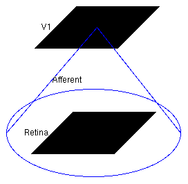
The large circle indicates that the Retina Sheet is fully connected to the V1 Sheet.
Initial weights
The plot below shows the initial set of weights from a 10x10 subset of the V1 neurons (i.e., every neuron with the reduced cortex_density, or every fourth neuron for cortex_density=40):
topo.sim.V1.Afferent.grid()

As we can see, the initial weights are uniform random. Each neuron receives a full set of connections from all input units, and thus each has a 24x24 or 10x10 array of weights (depending on the retina_density).
Initial Center-of-Gravity (CoG) plots
We can visualize the center of gravity (CoG) of the V1 Afferent weights using the following measurement command:
from topo.command.analysis import measure_cog
cog_data = measure_cog()
The center of gravity (a.k.a. centroid or center of mass) is computed for each neuron using its set of incoming weights. The plot below shows each neuron's CoG represented by a point, with a line segment drawn from each neuron to each of its four immediate neighbors so that neighborhood relationships (if any) will be visible.
cog_data.CoG.Afferent

From this plot is is clear that all of the neurons have a CoG near the center of the retina, which is to be expected because the weights are fully connected and evenly distributed (and thus all have an average (X,Y) value near the center of the retina). The same data is also visualized below:
xcog=cog_data.XCoG.Afferent.last
ycog=cog_data.YCoG.Afferent.last
xcog + ycog + xcog*ycog

The V1 X CoG plot shows the X location preferred by each neuron in V1, and the V1 Y CoG plot shows the preferred Y locations. The monochrome values are scaled so that a preference of -0.5 is black and a preference of +0.5 is white, and since they all start out around 0.0 they are all shades of medium gray. The actual preferences can be accessed directly as a Numpy array if you prefer:
xcog.data.min(),xcog.data.max(),ycog.data.min(),ycog.data.max()
The colorful XYCoG plot above right shows a false-color visualization of the CoG values in both dimensions at once, where the amount of red in the plot is proportional to the X CoG, and the amount of green in the plot is proportional to the Y CoG. Where both X and Y are low, the plot is black or very dark, and where both are high the plot is yellow (because red and green light together appears yellow). All of the units should be an intermediate color of yellow/gray at this stage, indicating preference for 0.5 in both X and Y. As you will see later, once neurons have developed strong preferences for one location over the others, some neurons will show up as bright black (X and Y both low), red (X high, Y low), red (X low, Y high), or yellow (X and Y both high) in this plot.
Training stimuli
We can have a look at what the training patterns that will be used to train the model without having to run it. In the cell labelled In [4] (in the model definition), we see where the training patterns are defined in a variable called input_pattern. We see that the circular Gaussian stimulus has x and y values that are drawn from a random distribution by two independent numbergen.UniformRandom objects. We can now view what 100 frames of training patterns will look like:
input_pattern.anim(30, offset=0.05)
Collecting data for animated plots
At the end of the notebook, we will generate a set of nice animations showing the plots we have already shown evolve over development. We now create a Collector object that collects all information needed for plotting and animation. We will collect the information we have just examined and advance the simulation one iteration:
from topo.analysis import Collector
from topo.command.analysis import measure_cog

c = Collector()
c.collect(measure_cog)

c.Activity.Retina     = c.collect(topo.sim.Retina)
c.Activity.V1         = c.collect(topo.sim.V1)
c.Activity.V1Afferent = c.collect(topo.sim.V1.Afferent)
c.CFs.Afferent        = c.collect(topo.sim.V1.Afferent, grid=True, rows=10, cols=10)
Activity after a single training iteration
The initial activities would be blank, but after running the model a single iteration, the sheet activities now look as follows:
data = c(times=[1])
data.Activity.Retina + data.Activity.V1

In the Retina plot, each photoreceptor is represented as a pixel whose shade of grey codes the response level, increasing from black to white. As expected, this particular example matches the first frame we visualized in the training stimulus animation. The V1 plot shows the response to that input, which for a SOM is initially a large Gaussian-shaped blob centered around the maximally responding unit.
Projection Activity
To see what the responses were before SOM’s neighborhood function forced them into a Gaussian shape, you can look at the Projection Activity plot, which shows the feedforward activity in V1:
data.Activity.V1Afferent

Here these responses are best thought of as Euclidean proximity, not distance. This formulation of the SOM response function actually subtracts the distances from the max distance, to ensure that the response will be larger for smaller Euclidean distances (as one intuitively expects for a neural response). The V1 feedforward activity appears random here because the Euclidean distance from the input vector to the initial random weight vector is random.
Learning after a few iterations
If you look at the weights now we have run a single training iteration, you'll see that most of the neurons have learned new weight patterns based on this input:
data.CFs.Afferent

Some of the weights to each neuron have now changed due to learning. In the SOM algorithm, the unit with the maximum response (i.e., the minimum Euclidean distance between its weight vector and the input pattern) is chosen, and the weights of units within a circular area defined by a Gaussian-shaped neighborhood function around this neuron are updated.
This effect is visible in this plot – a few neurons around the winning unit at the top right have changed their weights. Let us run a few more iterations before having another look:
topo.sim.run(4)
topo.sim.V1.Afferent.grid()

The weights have been updated again - it is clear after these five iterations that the input patterns are becoming represented in the weight patterns, though not very cleanly yet. We also see that the projection activity patterns are becoming smoother, since the weight vectors are now similar between neighboring neurons:
topo.sim.V1.Afferent.projection_view()

We will now advance to simulation time 250 because we will want to make animations regularly sampled every 250 steps:
topo.sim.run(245)
At 5000 iterations
Let us use our Collector object c to collect more measurements. We will start collecting measurements every 250 steps until we complete 5000 iterations, which should take a few seconds at the default densities, and may be a minute or two at the higher densities:
times = [topo.sim.time()*i for i in range(1,21)]
print("Running %d measurements between iteration %s and iteration %s" %
      (len(times), min(times), max(times)))
data = c(data, times=times)
We see that the topographic grid plot evolves over this period as follows:
data.CoG.Afferent
The X and Y CoG plots are now smooth, but not yet the axis-aligned gradients (e.g. left to right and bottom to top) that an optimal topographic mapping would have:
%%opts Image {-axiswise}
(data.XCoG.Afferent + data.YCoG.Afferent +
 data.XCoG.Afferent * data.YCoG.Afferent).select(Time=5000)

The weight patterns are still quite broad, not very selective for typical input patterns, and not very distinct from one another:
data.CFs.Afferent.last

In the live notebook you can remove the .last to view an animation to 5000 iterations
At 10000 iterations
Additional training up to 10000 iterations (which becomes faster due to a smaller neighborhood radius) leads to a nearly flat, square map:
times = [5000+(250*i) for i in range(1,21)]
print("Running %d measurements between iteration %s and iteration %s" %
      (len(times), min(times), max(times)))
data = c(data, times=times)
data.CoG.Afferent.last

Note: In the live notebook you can remove .last to view an animation to 10000 iterations
Note: In the live notebook you can remove .last to view an animation to 10000 iterations
Yet the weight patterns are still quite broad and not very selective for typical input patterns, because the neighborhood radius (initially 1.0 in Sheet coordinates, i.e. larger than the entire V1) is still large enough to force most cells to respond to the same patterns:
topo.sim.V1.output_fns[0].kernel_radius
data.CFs.Afferent.last

At 30000 iterations
By 30000 iterations the map has good coverage of the available portion of the input space:
times = [10000+(500*i) for i in range(1,41)]
print("Running %d measurements between iteration %s and iteration %s\n\n" %
      (len(times), min(times), max(times)))
data = c(data, times=times)
data.CoG.Afferent.last

The final projection plot at 30000 now shows that each neuron has developed weights concentrated in a small part of the input space, matching a prototypical input at one location, and that neurons each have distinct preferences:
topo.sim.V1.output_fns[0].kernel_radius
data.CFs.Afferent.last

The final topographic mapping may have any one of a number of possible arrangements, flipped or rotated by 90 degrees along any axis or both axes. E.g. a vertically flipped map will have blobs in each CF that are at the bottom for the top row of neurons, but the top for the bottom row of neurons. Nothing in the network reliably drives it to have any particular overall orientation or mapping apart from aligning to the square shape, and each of these possible organizations is equivalent functionally.
Animations over 30000 iterations
We can watch how the topographic mapping unfolds over all 30000 iterations we have run:
%%opts Gravity_Contours [rescale_individually=False]
data.CoG.Afferent
And how the XCoG and YCoG components unfold:
data.XCoG.Afferent + data.YCoG.Afferent + data.XCoG.Afferent * data.YCoG.Afferent
In the false color CoG plot, a perfectly organized mapping will have black in one corner and yellow in the opposite, with green and red in the two other corners, and smooth colors between each corner. Next, the weights (though by default this animation is disabled to save time, so you would need to remove ".last" and re-run this cell, which may take several minutes):
data.CFs.Afferent.last
Snapshots of the retinal and V1 activity over development. Notice how the activity in V1 becomes more focused over time as the kernel radius decreases:
data.Activity.Retina + data.Activity.V1
Exploring the parameters of the SOM
Now, you can re-run the basic simulation by restarting the IPython Notebook Kernel (Kernel -> Restart) or using the keyboard shortcut Ctrl+M . (see Help -> Keyboard Shortcuts for the full list). Then you can change one of the parameter values, either by editing the model definition above before running those cells, or (usually clearer) by setting the parameters in the cell labelled In [3].
For instance, the starting value of the neighborhood radius (from which all future values are calculated according to exponential decay) is 1.0. You can change this value as you see fit, e.g. to 0.1, by setting p.radius_0=0.1. With such a small learning radius, global ordering is unlikely to happen, and one can expect the topographic grid not to flatten out (despite local order in patches).
Similarly, consider changing the initial learning rate from 0.42 to e.g. 1.0 (e.g. by setting p.alpha_0=1.0 in cell 3). The retina and V1 densities cannot be changed after the simulation has started, but again, they can be changed by providing their values above and restarting the notebook.
You can also try changing the input_seed (p.input_seed=XX), to get a different stream of inputs, or weight_seed (p.weight_seed=XX), to get a different set of initial weights.
Note that with some of these values, you may encounter cases where the SOM fails to converge even though it seems to be working properly otherwise. For instance, some seed values result in topological defects like a kink:
%timer
Download this notebook from GitHub (right-click to download).